ML Practice 6_3

Dimensionaliy Reduction

: Decreasing the size of the data by selecting some features that best represent the data

  • To prevent overfitting and improve model performance
  • PCA(Principal Component Analysis), LDA(Linear Discriminant Analysis), etc

PCA

  • principal component(PC)
    • axis of data with the highest variance when projected on an axis
    • expressed as a linear combination of existing variables
    • Generally, it can be found as many as the features of the data as possible.
  • To explain the overall variation with 2 to 3 principal component

Import Data

1
2
3
4
!wget https://bit.ly/fruits_300_data -O fruits_300.npy
import numpy as np
fruits = np.load('fruits_300.npy')
fruits_2d = fruits.reshape(-1, 100*100)
--2022-03-31 06:10:20--  https://bit.ly/fruits_300_data
Resolving bit.ly (bit.ly)... 67.199.248.10, 67.199.248.11
Connecting to bit.ly (bit.ly)|67.199.248.10|:443... connected.
HTTP request sent, awaiting response... 301 Moved Permanently
Location: https://github.com/rickiepark/hg-mldl/raw/master/fruits_300.npy [following]
--2022-03-31 06:10:20--  https://github.com/rickiepark/hg-mldl/raw/master/fruits_300.npy
Resolving github.com (github.com)... 192.30.255.112
Connecting to github.com (github.com)|192.30.255.112|:443... connected.
HTTP request sent, awaiting response... 302 Found
Location: https://raw.githubusercontent.com/rickiepark/hg-mldl/master/fruits_300.npy [following]
--2022-03-31 06:10:20--  https://raw.githubusercontent.com/rickiepark/hg-mldl/master/fruits_300.npy
Resolving raw.githubusercontent.com (raw.githubusercontent.com)... 185.199.108.133, 185.199.111.133, 185.199.110.133, ...
Connecting to raw.githubusercontent.com (raw.githubusercontent.com)|185.199.108.133|:443... connected.
HTTP request sent, awaiting response... 200 OK
Length: 3000128 (2.9M) [application/octet-stream]
Saving to: ‘fruits_300.npy’

fruits_300.npy      100%[===================>]   2.86M  --.-KB/s    in 0.04s   

2022-03-31 06:10:21 (79.3 MB/s) - ‘fruits_300.npy’ saved [3000128/3000128]

PCA Model

1
2
3
4
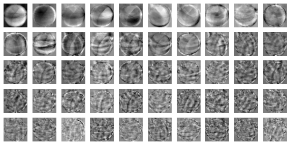
from sklearn.decomposition import PCA
pca = PCA(n_components=50)
pca.fit(fruits_2d)
print(pca.components_.shape)
(50, 10000)
1
2
3
4
5
6
7
8
9
10
11
12
13
14
import matplotlib.pyplot as plt

def draw_fruits(arr, ratio=1):
n = len(arr) # the number of sample
rows = int(np.ceil(n/10))
cols = n if rows < 2 else 10
fig, axs = plt.subplots(rows, cols,
figsize=(cols*ratio, rows*ratio), squeeze=False)
for i in range(rows):
for j in range(cols):
if i*10 + j < n: # n 개까지만 그립니다.
axs[i, j].imshow(arr[i*10 + j], cmap='gray_r')
axs[i, j].axis('off')
plt.show()
1
draw_fruits(pca.components_.reshape(-1, 100, 100))

1
2
3
print(fruits_2d.shape) # 10000 features
fruits_pca = pca.transform(fruits_2d)
print(fruits_pca.shape) # 50 features
(300, 10000)
(300, 50)
  • reduced to 1/200 compared to the original size of the data

Reconstruction of original data

1
2
3
4
fruits_inverse = pca.inverse_transform(fruits_pca)
print(fruits_inverse.shape)
fruits_reconstruct = fruits_inverse.reshape(-1, 100, 100)
print(fruits_reconstruct.shape)
(300, 10000)
(300, 100, 100)
1
draw_fruits(fruits_reconstruct[0:100])

1
draw_fruits(fruits_reconstruct[100:200])

1
draw_fruits(fruits_reconstruct[200:300])

  • Even though 10,000 features were reduced to 50, the original data were preserved fairly well.

Explained Variance

: How well the principal component represents the variance of the original data.

1
print(np.cumsum(pca.explained_variance_ratio_))
0.9215624972723878
[0.42357017 0.52298772 0.58876636 0.62907807 0.66324682 0.69606011
 0.72179277 0.7423424  0.75606517 0.76949289 0.78101436 0.79046031
 0.79924263 0.8077096  0.8146401  0.82109198 0.82688094 0.83199296
 0.83685678 0.84166025 0.8461386  0.85051178 0.85459218 0.85848695
 0.86221133 0.86580421 0.86911888 0.87229685 0.87534014 0.87837793
 0.8812672  0.88402533 0.88667509 0.88923363 0.89175254 0.8942257
 0.89662179 0.89893062 0.90115012 0.90331513 0.90544476 0.90740924
 0.90933715 0.91123892 0.91308592 0.91491101 0.91664894 0.91833369
 0.91995394 0.9215625 ]
1
2
3
fig, ax = plt.subplots()
ax.plot(pca.explained_variance_ratio_)
plt.show()

  • The first 10 PC represent most variance of the data.
  • Subsequent PC could hardly explain the variance of the data.

Use with other algorithms.

  • Logistic Regression of 3 classes
1
2
3
4
from sklearn.linear_model import LogisticRegression
lr = LogisticRegression()

target = np.array([0]*100 + [1]*100 + [2]*100) # create target values
  • cross-validation with original data
1
2
3
4
from sklearn.model_selection import cross_validate
scores = cross_validate(lr, fruits_2d, target)
print(np.mean(scores['test_score']))
print(np.mean(scores['fit_time']))
0.9966666666666667
1.511155652999878
  • cross-validation with reduced data in PCA
1
2
3
scores = cross_validate(lr, fruits_pca, target)
print(np.mean(scores['test_score']))
print(np.mean(scores['fit_time']))
1.0
0.07492985725402831

Specify the variance ratio

1
2
3
pca = PCA(n_components=0.5)
pca.fit(fruits_2d)
print(pca.n_components_) # 2 PC needed
2
1
2
fruits_pca = pca.transform(fruits_2d)
print(fruits_pca.shape)
(300, 2)
1
2
3
scores = cross_validate(lr, fruits_pca, target)
print(np.mean(scores['test_score']))
print(np.mean(scores['fit_time']))
0.9933333333333334
0.03829236030578613


/usr/local/lib/python3.7/dist-packages/sklearn/linear_model/_logistic.py:818: ConvergenceWarning: lbfgs failed to converge (status=1):
STOP: TOTAL NO. of ITERATIONS REACHED LIMIT.

Increase the number of iterations (max_iter) or scale the data as shown in:
    https://scikit-learn.org/stable/modules/preprocessing.html
Please also refer to the documentation for alternative solver options:
    https://scikit-learn.org/stable/modules/linear_model.html#logistic-regression
  extra_warning_msg=_LOGISTIC_SOLVER_CONVERGENCE_MSG,
1
2
3
4
5
from sklearn.cluster import KMeans
km = KMeans(n_clusters=3, random_state=42)
km.fit(fruits_pca)
print(np.unique(km.labels_, return_counts=True))
# label 0: 110 / label 1: 99 / label 2: 91
(array([0, 1, 2], dtype=int32), array([110,  99,  91]))
1
draw_fruits(fruits[km.labels_==0])

1
draw_fruits(fruits[km.labels_==1])

1
draw_fruits(fruits[km.labels_==2])

1
2
3
4
5
6
fig, ax = plt.subplots()
for label in range(3):
data = fruits_pca[km.labels_==label]
ax.scatter(data[:,0], data[:,1])
ax.legend(['apple','banana','pineapple'])
plt.show()

Ref.) 혼자 공부하는 머신러닝+딥러닝 (박해선, 한빛미디어)

Share