Prepare Data
Import wine data set
class 0: red wine
class 1: white wine
1
2
3
import pandas as pdwine = pd.read_csv("https://bit.ly/wine_csv_data" ) print (wine.head())
   alcohol  sugar    pH  class
0      9.4    1.9  3.51    0.0
1      9.8    2.6  3.20    0.0
2      9.8    2.3  3.26    0.0
3      9.8    1.9  3.16    0.0
4      9.4    1.9  3.51    0.0
<class 'pandas.core.frame.DataFrame'>
RangeIndex: 6497 entries, 0 to 6496
Data columns (total 4 columns):
# Column Non-Null Count Dtype
--- ------ -------------- -----
0 alcohol 6497 non-null float64
1 sugar 6497 non-null float64
2 pH 6497 non-null float64
3 class 6497 non-null float64
dtypes: float64(4)
memory usage: 203.2 KB
alcohol sugar pH class
count 6497.000000 6497.000000 6497.000000 6497.000000
mean 10.491801 5.443235 3.218501 0.753886
std 1.192712 4.757804 0.160787 0.430779
min 8.000000 0.600000 2.720000 0.000000
25% 9.500000 1.800000 3.110000 1.000000
50% 10.300000 3.000000 3.210000 1.000000
75% 11.300000 8.100000 3.320000 1.000000
max 14.900000 65.800000 4.010000 1.000000
Split data into training sets and test sets
1 2 data = wine[['alcohol' , 'sugar' , 'pH' ]].to_numpy() target = wine['class' ].to_numpy()
1 2 3 4 5 from sklearn.model_selection import train_test_splittrain_input, test_input, train_target, test_target = train_test_split( data, target, test_size=0.2 , random_state=42 ) print (train_input.shape, test_input.shape)
(5197, 3) (1300, 3)
Standardize Data
Decision tree does not require standardized preprocessing,
1
2
3
4
5
from sklearn.preprocessing import StandardScalerss = StandardScaler() ss.fit(train_input) train_scaled = ss.transform(train_input) test_scaled = ss.transform(test_input)
Logistic Regression Model 1 2 3 4 5 from sklearn.linear_model import LogisticRegressionlr = LogisticRegression() lr.fit(train_scaled, train_target) print (lr.score(train_scaled, train_target))print (lr.score(test_scaled, test_target))
0.7808350971714451
0.7776923076923077
1 2 print (lr.predict_proba(train_scaled[:5 ]))print (lr.predict(train_scaled[:5 ]))
[[0.06189333 0.93810667]
[0.21742616 0.78257384]
[0.40703571 0.59296429]
[0.45226659 0.54773341]
[0.00530794 0.99469206]]
[1. 1. 1. 1. 1.]
1 print (lr.coef_, lr.intercept_)
[[ 0.51270274 1.6733911 -0.68767781]] [1.81777902]
Decision Tree Model : a non-parametric supervised learning method used for classification and regression
to predict the value of a target variable by learning simple decision rules inferred from the data features
Simple to understand and to interpret
More likely to be overfitting the training set.
New Algorithm Using Decision Tree Algorithms
XGBoost, LightGBM, CatBoost, etc
In particular, LightGBM is now widely used in practice.
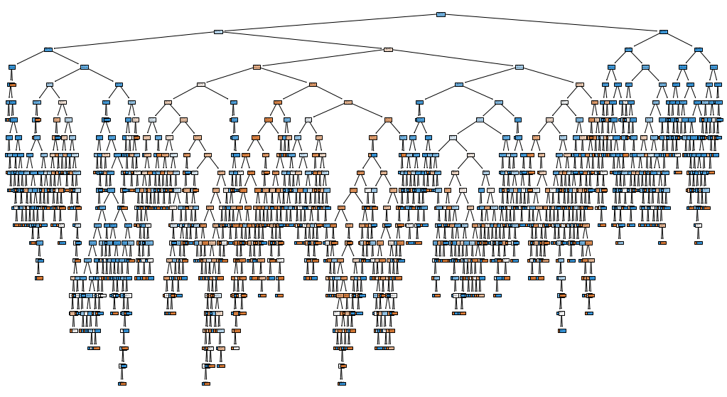
DecisionTreeClassifier 1 2 3 4 5 from sklearn.tree import DecisionTreeClassifierdt = DecisionTreeClassifier(random_state=42 ) dt.fit(train_scaled, train_target) print (dt.score(train_scaled, train_target))print (dt.score(test_scaled, test_target))
0.996921300750433
0.8592307692307692
1 2 3 4 5 6 7 8 9 10 import matplotlib.pyplot as pltfrom sklearn.tree import plot_treefig, ax = plt.subplots(figsize=(18 ,10 )) plot_tree(dt, filled=True , feature_names=['alcohol' ,'sugar' ,'pH' ]) plt.show()
Impurity(불순도)
parameter criterion; default ‘gini’
gini = 1 - (negative_prop^2 + positive_prop^2)
best : 0 (pure node)
worst : 0.5 (exactly half and half)
entropy = - negative_prop * log_2(negative_prop) - positive_prop * log_2(positive_prop)
Information gain(정보 이득) : impurity differences between parent node and child node
Decision tree splits nodes to maximize information gain using impurity criteria.
Pruning(가지치기)
In order to prevent overfitting the training set
By specifying the maximum depth of a tree that can grow
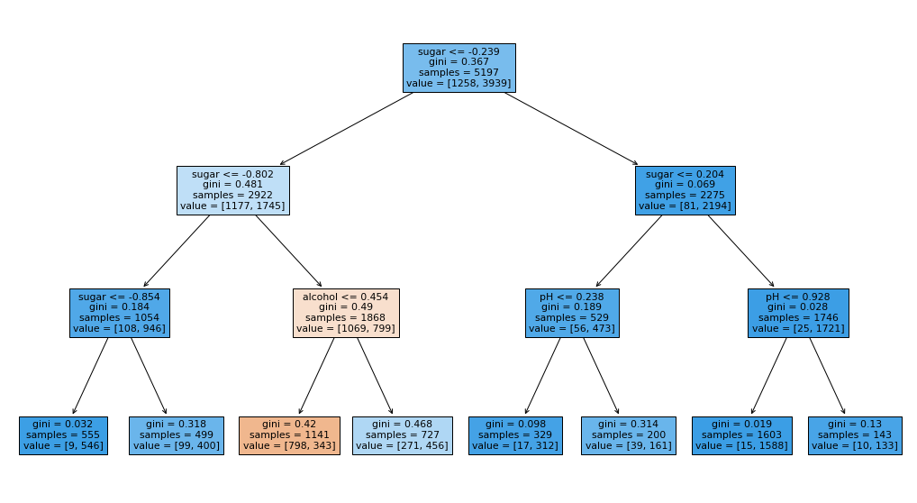
1 2 3 4 dt = DecisionTreeClassifier(max_depth=3 , random_state=42 ) dt.fit(train_scaled, train_target) print (dt.score(train_scaled, train_target))print (dt.score(test_scaled, test_target))
0.8454877814123533
0.8415384615384616
1 2 3 fig, ax = plt.subplots(figsize=(18 ,10 )) plot_tree(dt, filled=True , feature_names=['alcohol' ,'sugar' ,'pH' ]) plt.show()
1 2 3 4 5 6 7 8 9 import graphvizfrom sklearn import treedot_data = tree.export_graphviz( dt, out_file=None , feature_names = ['alcohol' ,'sugar' ,'pH' ], filled=True ) graph = graphviz.Source(dot_data, format ="png" ) graph
1 graph.render("decision_tree_graphivz" )
'decision_tree_graphivz.png'
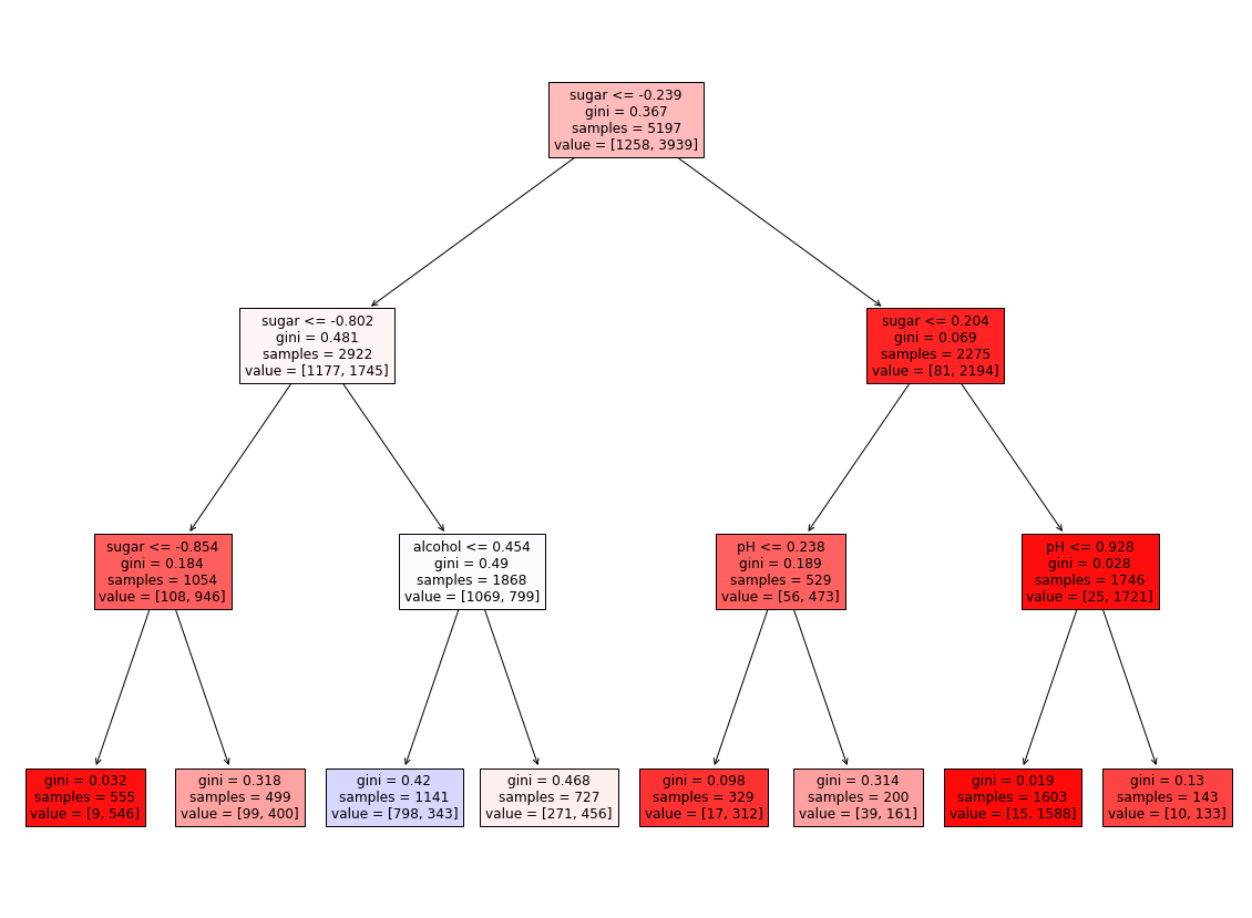
1 2 3 4 5 6 7 8 9 10 11 12 13 14 15 16 from matplotlib.colors import ListedColormap, to_rgbimport numpy as npplt.figure(figsize=(20 , 15 )) artists = plot_tree(dt, filled = True , feature_names = ['alcohol' ,'sugar' ,'pH' ]) colors = ['blue' , 'red' ] for artist, impurity, value in zip (artists, dt.tree_.impurity, dt.tree_.value): r, g, b = to_rgb(colors[np.argmax(value)]) f = impurity * 2 artist.get_bbox_patch().set_facecolor((f + (1 -f)*r, f + (1 -f)*g, f + (1 -f)*b)) artist.get_bbox_patch().set_edgecolor('black' ) plt.show()
parameter min_impurity_decrease; default 0.0
Split nodes if this split induces a decrease of the impurity greater than or equal to this value.
More likely to be asymmetric tree
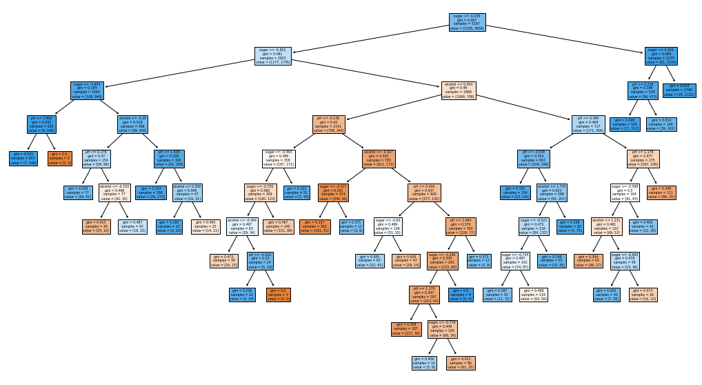
1 2 3 4 5 6 7 8 dt = DecisionTreeClassifier(min_impurity_decrease=0.0005 , random_state=42 ) dt.fit(train_scaled, train_target) print (dt.score(train_scaled, train_target))print (dt.score(test_scaled, test_target))fig, ax = plt.subplots(figsize=(18 , 10 )) plot_tree(dt, filled=True , feature_names=['alcohol' ,'sugar' ,'pH' ]) plt.show()
0.8874350586877044
0.8615384615384616
Feature importance : an indicator of the degree to which each feature contributed to reducing impurities
Multiply the information gain and the ratio of the total sample by each node, and add it up by feature.
1 print (dt.feature_importances_)
[0.12345626 0.86862934 0.0079144 ]
Ref.) 혼자 공부하는 머신러닝+딥러닝 (박해선, 한빛미디어)