Prepare Data Import data set 1 2 3 4 import pandas as pdfish = pd.read_csv('https://bit.ly/fish_csv_data' ) print (fish.head())
Species Weight Length Diagonal Height Width
0 Bream 242.0 25.4 30.0 11.5200 4.0200
1 Bream 290.0 26.3 31.2 12.4800 4.3056
2 Bream 340.0 26.5 31.1 12.3778 4.6961
3 Bream 363.0 29.0 33.5 12.7300 4.4555
4 Bream 430.0 29.0 34.0 12.4440 5.1340
1 print (pd.unique(fish['Species' ]))
['Bream' 'Roach' 'Whitefish' 'Parkki' 'Perch' 'Pike' 'Smelt']
Convert to Numpy array 1 2 3 fish_input = fish[['Weight' ,'Length' ,'Diagonal' ,'Height' ,'Width' ]].to_numpy() print (fish_input.shape)print (fish_input[:3 ])
(159, 5)
[[242. 25.4 30. 11.52 4.02 ]
[290. 26.3 31.2 12.48 4.3056]
[340. 26.5 31.1 12.3778 4.6961]]
1 2 fish_target = fish['Species' ].to_numpy() print (fish_target.shape)
(159,)
Split and Standardize 1 2 3 4 from sklearn.model_selection import train_test_splittrain_input, test_input, train_target, test_target = train_test_split( fish_input, fish_target, random_state=42 )
1 2 3 4 5 from sklearn.preprocessing import StandardScalerss = StandardScaler() ss.fit(train_input) train_scaled = ss.transform(train_input) test_scaled = ss.transform(test_input)
1 2 print (train_input[:3 ])print (train_scaled[:3 ])
[[720. 35. 40.6 16.3618 6.09 ]
[500. 45. 48. 6.96 4.896 ]
[ 7.5 10.5 11.6 1.972 1.16 ]]
[[ 0.91965782 0.60943175 0.81041221 1.85194896 1.00075672]
[ 0.30041219 1.54653445 1.45316551 -0.46981663 0.27291745]
[-1.0858536 -1.68646987 -1.70848587 -1.70159849 -2.0044758 ]
[-0.79734143 -0.60880176 -0.67486907 -0.82480589 -0.27631471]
[-0.71289885 -0.73062511 -0.70092664 -0.0802298 -0.7033869 ]]
[[-0.88741352 -0.91804565 -1.03098914 -0.90464451 -0.80762518]
[-1.06924656 -1.50842035 -1.54345461 -1.58849582 -1.93803151]
[-0.54401367 0.35641402 0.30663259 -0.8135697 -0.65388895]
[-0.34698097 -0.23396068 -0.22320459 -0.11905019 -0.12233464]
[-0.68475132 -0.51509149 -0.58801052 -0.8998784 -0.50124996]]
KNN Classifier Model fitting 1 2 3 4 5 6 7 from sklearn.neighbors import KNeighborsClassifierkn = KNeighborsClassifier(n_neighbors=3 ) kn.fit(train_scaled, train_target) print (kn.score(train_scaled, train_target))print (kn.score(test_scaled, test_target))
0.8907563025210085
0.85
Multi-class Classfication 1 2 3 4 import numpy as npproba = kn.predict_proba(test_scaled[:5 ]) print (kn.classes_)print (np.round (proba, decimals=4 ))
['Bream' 'Parkki' 'Perch' 'Pike' 'Roach' 'Smelt' 'Whitefish']
[[0. 0. 1. 0. 0. 0. 0. ]
[0. 0. 0. 0. 0. 1. 0. ]
[0. 0. 0. 1. 0. 0. 0. ]
[0. 0. 0.6667 0. 0.3333 0. 0. ]
[0. 0. 0.6667 0. 0.3333 0. 0. ]]
1 2 distances, indexes = kn.kneighbors(test_scaled[3 :4 ]) print (train_target[indexes])
[['Roach' 'Perch' 'Perch']]
The probability calculated by the model is the ratio of the nearest neighbor.
In this model(k=3), the probability values are 0, 1/3, 2/3, and 1.
If k is set as 5, the probability values may be 0, 0.2, 0.4, 0.6, 0.8 and 1.
1 2 3 4 5 6 kn = KNeighborsClassifier(n_neighbors=5 ) kn.fit(train_scaled, train_target) proba = kn.predict_proba(test_scaled[:5 ]) print (kn.classes_)print (np.round (proba, decimals=4 ))print (kn.predict(test_scaled[:5 ]))
['Bream' 'Parkki' 'Perch' 'Pike' 'Roach' 'Smelt' 'Whitefish']
[[0. 0. 0.6 0. 0.4 0. 0. ]
[0. 0. 0. 0. 0. 1. 0. ]
[0. 0. 0.2 0.8 0. 0. 0. ]
[0. 0. 0.8 0. 0.2 0. 0. ]
[0. 0. 0.8 0. 0.2 0. 0. ]]
['Perch' 'Smelt' 'Pike' 'Perch' 'Perch']
Logistic Regression : Estimating a model with a regression equation for categorical dependent variables.
Despite its name, a classification model rather than regression model
Highly important model
used as basic statistics (especially medical statistics)
the basis of the machine learning classification model.
early model of deep learning
To overcome the linearity assumption problem of general regression equation
Logit transformation : the log of the odds ratio
Using the logit of Y as the dependent variable of the regression
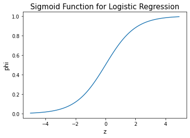
Sigmoid function
also called a logistic function
Convert the value z calculated by linear regression to a probability value between 0 and 1
z < 0: the function approaches 0
z > 0: the function approaches 1
z = 0: the function value is 0.5
1 2 3 4 5 6 7 8 9 10 11 import numpy as npimport matplotlib.pyplot as pltz = np.arange(-5 , 5 , 0.1 ) phi = 1 / (1 + np.exp(-z)) fig, ax = plt.subplots() ax.plot(z, phi) ax.set_xlabel('z' , fontsize=12 ) ax.set_ylabel('phi' , fontsize=12 ) ax.set_title("Sigmoid Function for Logistic Regression" , fontsize=15 ) plt.show()
Binary classification 1 2 3 4 5 bream_smelt_indexes = (train_target == 'Bream' ) | (train_target == 'Smelt' ) train_bream_smelt = train_scaled[bream_smelt_indexes] target_bream_smelt = train_target[bream_smelt_indexes]
1 2 3 4 5 6 7 8 from sklearn.linear_model import LogisticRegressionlr = LogisticRegression() lr.fit(train_bream_smelt, target_bream_smelt) print (lr.classes_) proba = lr.predict_proba(train_bream_smelt[:5 ]) print (np.round (proba, decimals=3 )) print (lr.predict(train_bream_smelt[:5 ]))
['Bream' 'Smelt']
[[0.998 0.002]
[0.027 0.973]
[0.995 0.005]
[0.986 0.014]
[0.998 0.002]]
['Bream' 'Smelt' 'Bream' 'Bream' 'Bream']
1 print (lr.coef_, lr.intercept_)
[[-0.4037798 -0.57620209 -0.66280298 -1.01290277 -0.73168947]] [-2.16155132]
z = - 0.404 * Weight - 0. 576 * Length - 0.663 * Diagonal - 1.013 * Height - 0.732 * Width - 2.162
1 2 decisions = lr.decision_function(train_bream_smelt[:5 ]) print (decisions)
[-6.02927744 3.57123907 -5.26568906 -4.24321775 -6.0607117 ]
1 2 from scipy.special import expitprint (expit(decisions))
[0.00240145 0.97264817 0.00513928 0.01415798 0.00232731]
Multi-class classification
basically use iterative algorithms (max_iter, default 100)
in this model, set max_iter as 1000 (for sufficient training)
L2 Regularization
based on the square value of the coefficient such as ridge regression
hyperparameter; C ( default 1)
the smaller the value, the greater the regulation.
in this model, set C as 20 (in order to ease regulations a little)
1 2 3 4 lr = LogisticRegression(C=20 , max_iter=1000 ) lr.fit(train_scaled, train_target) print (lr.score(train_scaled, train_target))print (lr.score(test_scaled, test_target))
0.9327731092436975
0.925
1 2 3 4 print (lr.classes_)proba = lr.predict_proba(test_scaled[:5 ]) print (np.round (proba, decimals=3 )) print (lr.predict(test_scaled[:5 ]))
['Bream' 'Parkki' 'Perch' 'Pike' 'Roach' 'Smelt' 'Whitefish']
[[0. 0.014 0.841 0. 0.136 0.007 0.003]
[0. 0.003 0.044 0. 0.007 0.946 0. ]
[0. 0. 0.034 0.935 0.015 0.016 0. ]
[0.011 0.034 0.306 0.007 0.567 0. 0.076]
[0. 0. 0.904 0.002 0.089 0.002 0.001]]
['Perch' 'Smelt' 'Pike' 'Roach' 'Perch']
1 print (lr.coef_.shape, lr.intercept_.shape)
(7, 5) (7,)
[[-1.49002087 -1.02912886 2.59345551 7.70357682 -1.2007011 ]
[ 0.19618235 -2.01068181 -3.77976834 6.50491489 -1.99482722]
[ 3.56279745 6.34357182 -8.48971143 -5.75757348 3.79307308]
[-0.10458098 3.60319431 3.93067812 -3.61736674 -1.75069691]
[-1.40061442 -6.07503434 5.25969314 -0.87220069 1.86043659]
[-1.38526214 1.49214574 1.39226167 -5.67734118 -4.40097523]
[ 0.62149861 -2.32406685 -0.90660867 1.71599038 3.6936908 ]]
[-0.09205179 -0.26290885 3.25101327 -0.14742956 2.65498283 -6.78782948
1.38422358]
The z value is calculated one by one for each class and classified into the class that outputs the highest value.
Softmax function
also called a normalized exponential function (because of using exponential functions)
The outputs of several linear equations are compressed from 0 to 1, and the total sum is 1.
e_sum = e^z1 + e^z2 + … + e^z7
s1 = e^z1/e_sum, s2 = e^z2/e_sum, … , s7 = e^z7/e_sum
1 2 decision = lr.decision_function(test_scaled[:5 ]) print (np.round (decision, decimals=3 ))
[[ -6.498 1.032 5.164 -2.729 3.339 0.327 -0.634]
[-10.859 1.927 4.771 -2.398 2.978 7.841 -4.26 ]
[ -4.335 -6.233 3.174 6.487 2.358 2.421 -3.872]
[ -0.683 0.453 2.647 -1.187 3.265 -5.753 1.259]
[ -6.397 -1.993 5.816 -0.11 3.503 -0.112 -0.707]]
1 2 3 from scipy.special import softmaxproba = softmax(decision, axis=1 ) print (np.round (proba, decimals=3 ))
[[0.    0.014 0.841 0.    0.136 0.007 0.003]
 [0.    0.003 0.044 0.    0.007 0.946 0.   ]
 [0.    0.    0.034 0.935 0.015 0.016 0.   ]
 [0.011 0.034 0.306 0.007 0.567 0.    0.076]
 [0.    0.    0.904 0.002 0.089 0.002 0.001]]
Ref.) 혼자 공부하는 머신러닝+딥러닝 (박해선, 한빛미디어)