Prepare Data 1 2 3 import pandas as pddf = pd.read_csv('https://bit.ly/perch_csv_data' ) perch_full = df.to_numpy()
1 2 3 4 5 6 7 8 import numpy as npperch_weight = np.array([5.9 , 32.0 , 40.0 , 51.5 , 70.0 , 100.0 , 78.0 , 80.0 , 85.0 , 85.0 , 110.0 , 115.0 , 125.0 , 130.0 , 120.0 , 120.0 , 130.0 , 135.0 , 110.0 , 130.0 , 150.0 , 145.0 , 150.0 , 170.0 , 225.0 , 145.0 , 188.0 , 180.0 , 197.0 , 218.0 , 300.0 , 260.0 , 265.0 , 250.0 , 250.0 , 300.0 , 320.0 , 514.0 , 556.0 , 840.0 , 685.0 , 700.0 , 700.0 , 690.0 , 900.0 , 650.0 , 820.0 , 850.0 , 900.0 , 1015.0 , 820.0 , 1100.0 , 1000.0 , 1100.0 , 1000.0 , 1000.0 ])
1 2 3 4 from sklearn.model_selection import train_test_splittrain_input, test_input, train_target, test_target = train_test_split( perch_full, perch_weight, random_state=42 )
※ Scikit-Learn Class
Estimator(추정기; model class) : Fitting and predicting
KNeighborsClassifier, LinearRegression, etc.
common method : fit(), score(), predict()
Transformer(변환기) and Pre-processors : transforming or imputing data
PolynomialFeatures, StandardScaler, etc
common method : fit(), transform()
※ Feature engineering(특성 공학)
extracting new features using existing features
existing features, square features of each, and features multiplied by each other.
1 from sklearn.preprocessing import PolynomialFeatures
1 2 3 poly = PolynomialFeatures() poly.fit([[2 ,3 ]]) print (poly.transform([[2 ,3 ]]))
[[1. 2. 3. 4. 6. 9.]]
> existing features : 2, 3
> new features : 1(for intercept), 4(2^2), 6(2*3), 9(3^2)
case 2: Not including a bias (recommended)
1 2 3 poly = PolynomialFeatures(include_bias=False ) poly.fit([[2 ,3 ]]) print (poly.transform([[2 ,3 ]]))
[[2. 3. 4. 6. 9.]]
> existing features : 2, 3
> new features : 4(2^2), 6(2*3), 9(3^2)
1 2 3 4 5 6 7 poly = PolynomialFeatures(include_bias=False ) poly.fit(train_input) train_poly = poly.transform(train_input) print (train_input.shape) print (train_poly.shape) print (poly.get_feature_names_out())
(42, 3)
(42, 9)
['x0' 'x1' 'x2' 'x0^2' 'x0 x1' 'x0 x2' 'x1^2' 'x1 x2' 'x2^2']
1 2 3 test_poly = poly.transform(test_input) print (test_input.shape) print (test_poly.shape)
(14, 3)
(14, 9)
Mutiple Regression
same process as training a linear regression model
linear regression using multiple features
degree 2 1 2 3 4 5 from sklearn.linear_model import LinearRegressionlr = LinearRegression() lr.fit(train_poly, train_target) print (lr.score(train_poly, train_target))print (lr.score(test_poly, test_target))
0.9903183436982124
0.9714559911594134
Multiple regression solves the linear model’s underfitting problem.
The score for the training set is very high.
degree 5 1 2 3 4 5 6 poly = PolynomialFeatures(degree=5 , include_bias=False ) poly.fit(train_input) train_poly = poly.transform(train_input) test_poly = poly.transform(test_input) print (train_poly.shape)print (test_poly.shape)
(42, 55)
(14, 55)
1 2 3 lr.fit(train_poly, train_target) print (lr.score(train_poly, train_target))print (lr.score(test_poly, test_target))
0.9999999999991097
-144.40579242684848
The score for the training set is almost perfect.
But the score for the testing set is extremely negative.
The model appears to be too overfitting to the training set.
Regularization(규제)
preventing the model from overfitting the training set
linear regression model : reducing the size of the coefficient multiplied by the feature.
hyperparameter: alpha
parameter which has to be set in advance
increase/decrease in regulatory intensity
adjusted to increase the performance of the model
Conceptual understanding is important, but it doesn’t mean much in practice.
No guarantee of performance compared to working hours.
More than 100 libraries in scikit-learn, and the types and numbers of hyperparameters vary.
Better to use the existing hyperparameters, for unfamiliar models.
Normalize feature scales
using StandardScaler class in scikit-learn
1 2 3 4 5 6 7 from sklearn.preprocessing import StandardScalerss = StandardScaler() ss.fit(train_poly) train_scaled = ss.transform(train_poly) test_scaled = ss.transform(test_poly) print (train_poly.shape)print (test_poly.shape)
(42, 55)
(14, 55)
Ridge regression
based on the square value of the coefficient
1 2 3 4 5 from sklearn.linear_model import Ridgeridge = Ridge() ridge.fit(train_scaled, train_target) print (ridge.score(train_scaled, train_target))print (ridge.score(test_scaled, test_target))
0.9896101671037343
0.9790693977615397
Many features are used, but they’re not overfitting the training set and perform well on the test set.
1 2 3 import matplotlib.pyplot as plttrain_score = [] test_score = []
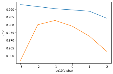
1 2 3 4 5 6 alpha_list = [0.001 , 0.01 , 0.1 , 1 , 10 , 100 ] for alpha in alpha_list: ridge = Ridge(alpha=alpha) ridge.fit(train_scaled, train_target) train_score.append(ridge.score(train_scaled, train_target)) test_score.append(ridge.score(test_scaled, test_target))
1 2 3 4 5 6 fig, ax = plt.subplots() ax.plot(np.log10(alpha_list), train_score) ax.plot(np.log10(alpha_list), test_score) ax.set_xlabel('log10(alpha)' ) ax.set_ylabel('R^2' ) plt.show()
left side : overfitting
right side : underfitting
appropriate alpha : 0.1
1 2 3 4 ridge = Ridge(alpha=0.1 ) ridge.fit(train_scaled, train_target) print (ridge.score(train_scaled, train_target))print (ridge.score(test_scaled, test_target))
0.9903815817570366
0.9827976465386926
Lasso regression
based on the absolute value of the coefficient
The coefficient can be completely zero.
1 2 3 4 5 from sklearn.linear_model import Lassolasso = Lasso() lasso.fit(train_scaled, train_target) print (lasso.score(train_scaled, train_target))print (lasso.score(test_scaled, test_target))
0.989789897208096
0.9800593698421883
Many features are used, but they’re not overfitting the training set and perform well on the test set.
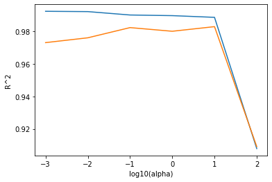
1 2 3 4 5 6 7 8 9 train_score = [] test_score = [] alpha_list = [0.001 , 0.01 , 0.1 , 1 , 10 , 100 ] for alpha in alpha_list: lasso = Lasso(alpha=alpha, max_iter=10000 ) lasso.fit(train_scaled, train_target) train_score.append(lasso.score(train_scaled, train_target)) test_score.append(lasso.score(test_scaled, test_target))
/usr/local/lib/python3.7/dist-packages/sklearn/linear_model/_coordinate_descent.py:648: ConvergenceWarning: Objective did not converge. You might want to increase the number of iterations, check the scale of the features or consider increasing regularisation. Duality gap: 1.878e+04, tolerance: 5.183e+02
coef_, l1_reg, l2_reg, X, y, max_iter, tol, rng, random, positive
/usr/local/lib/python3.7/dist-packages/sklearn/linear_model/_coordinate_descent.py:648: ConvergenceWarning: Objective did not converge. You might want to increase the number of iterations, check the scale of the features or consider increasing regularisation. Duality gap: 1.297e+04, tolerance: 5.183e+02
coef_, l1_reg, l2_reg, X, y, max_iter, tol, rng, random, positive
1 2 3 4 5 6 fig, ax = plt.subplots() ax.plot(np.log10(alpha_list), train_score) ax.plot(np.log10(alpha_list), test_score) ax.set_xlabel('log10(alpha)' ) ax.set_ylabel('R^2' ) plt.show()
left side : overfitting
right side : underfitting
appropriate alpha : 10
1 2 3 4 lasso = Lasso(alpha=10 ) lasso.fit(train_scaled, train_target) print (lasso.score(train_scaled, train_target))print (lasso.score(test_scaled, test_target))
0.9888067471131867
0.9824470598706695
1 print (np.sum (lasso.coef_==0 ))
40
40 coefficients became zero
Of the 55 features, only 15 were finally used.
Ref.) 혼자 공부하는 머신러닝+딥러닝 (박해선, 한빛미디어)