Data Set
1 | import numpy as np |
1 | from sklearn.model_selection import train_test_split |
((42,), (14,), (42,), (14,))
1 | train_input = train_input.reshape(-1,1) |
(42, 1) (14, 1)
KNN Regression
1 | from sklearn.neighbors import KNeighborsRegressor |
0.9746459963987609
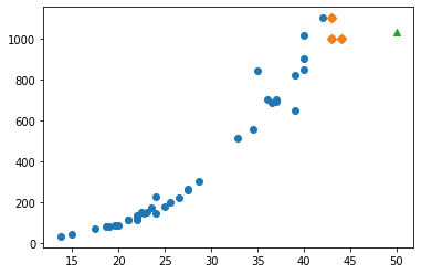
Predict a data 1
- the weight of a 50-centimeter-long perch
1 | print(knr.predict([[50]])) |
[1033.33333333]
1 | import matplotlib.pyplot as plt |
Predict a data 2
- the weight of a 100-centimeter-long perch
1 | print(knr.predict([[100]])) |
[1033.33333333]
1 | distances, indexes = knr.kneighbors([[100]]) |
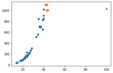
Beyond the scope of the new training set, incorrect values can be predicted.
No matter how big the length is, the weight doesn’t increase anymore.
※ Machine learning models must be trained periodically.
MLOps (Machine Learning & Opearations)
- the essential skill for data scientist, ML engineer.
Linear Regression
- in statistics:
- The process of finding causal relationships is more important.
- 4 assumptions (linearity, normality, independence, equal variance)
- in ML:
- Predicting results is more important.
- R-squared, MAE, RMSE, etc
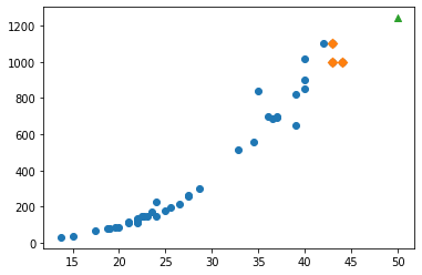
Predict a data
1 | from sklearn.linear_model import LinearRegression |
[1241.83860323]
1 | fig, ax = plt.subplots() |
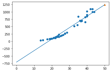
Regression equation
- coef_ : regression coefficient(weight)
- intercept_ : regression intercept
$y = a + bx$
- coefficient & intercept : model parameter
- Linear Regression is a model-based learning.
- KNN Regression is a case-based learning.
1 | print(lr.coef_, lr.intercept_) |
[39.01714496] -709.0186449535477
1 | fig, ax = plt.subplots() |
1 | print(lr.score(train_input, train_target)) |
0.939846333997604
0.8247503123313558
- The model is so simple that it is underfit overall.
- It seems that polynomial regression is needed.
Polynomial Regression
- coef_ : regression coefficients(weights)
- intercept_ : regression intercept
$y = a + b_1x_1 + b_2x_2 + … + b_nx_n$
Predict a data
1 | # Broadcasting in Numpy |
(42, 2) (14, 2)
※ Broadcasting in Numpy
1 | lr2 = LinearRegression() |
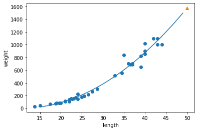
[1573.98423528]
Regression equation
1 | print(lr2.coef_, lr2.intercept_) |
[ 1.01433211 -21.55792498] 116.0502107827827
1 | point = np.arange(15,50) |
1 | print(lr2.score(train_poly, train_target)) |
0.9706807451768623
0.9775935108325122
- The model has improved a lot, but it is still underfit.
- It seems that a more complex model is needed.
Ref.) 혼자 공부하는 머신러닝+딥러닝 (박해선, 한빛미디어)