ML Practice 2_2

Prepare data with Numpy

fish_length = [25.4, 26.3, 26.5, 29.0, 29.0, 29.7, 29.7, 30.0, 30.0, 30.7, 31.0, 31.0, 
                31.5, 32.0, 32.0, 32.0, 33.0, 33.0, 33.5, 33.5, 34.0, 34.0, 34.5, 35.0, 
                35.0, 35.0, 35.0, 36.0, 36.0, 37.0, 38.5, 38.5, 39.5, 41.0, 41.0, 9.8, 
                10.5, 10.6, 11.0, 11.2, 11.3, 11.8, 11.8, 12.0, 12.2, 12.4, 13.0, 14.3, 15.0]
fish_weight = [242.0, 290.0, 340.0, 363.0, 430.0, 450.0, 500.0, 390.0, 450.0, 500.0, 475.0, 500.0, 
                500.0, 340.0, 600.0, 600.0, 700.0, 700.0, 610.0, 650.0, 575.0, 685.0, 620.0, 680.0, 
                700.0, 725.0, 720.0, 714.0, 850.0, 1000.0, 920.0, 955.0, 925.0, 975.0, 950.0, 6.7, 
                7.5, 7.0, 9.7, 9.8, 8.7, 10.0, 9.9, 9.8, 12.2, 13.4, 12.2, 19.7, 19.9]

import numpy as np
fish_data = np.column_stack((fish_length, fish_weight))
print(fish_data[:5])

[[ 25.4 242. ]
 [ 26.3 290. ]
 [ 26.5 340. ]
 [ 29.  363. ]
 [ 29.  430. ]]

fish_target = np.concatenate((np.ones(35), np.zeros(14)))
print(fish_target)

[1. 1. 1. 1. 1. 1. 1. 1. 1. 1. 1. 1. 1. 1. 1. 1. 1. 1. 1. 1. 1. 1. 1. 1.
 1. 1. 1. 1. 1. 1. 1. 1. 1. 1. 1. 0. 0. 0. 0. 0. 0. 0. 0. 0. 0. 0. 0. 0.
 0.]

Split data with Scikit-learn

from sklearn.model_selection import train_test_split

# stratify: spliting data according to class proportions
train_input, test_input, train_target, test_target = train_test_split(fish_data, fish_target, stratify=fish_target, random_state=42)

print(train_input.shape, test_input.shape)
print(train_target.shape, test_target.shape)
print(test_target)

(36, 2) (13, 2)
(36,) (13,)
[0. 0. 1. 0. 1. 0. 1. 1. 1. 1. 1. 1. 1.]

KNN 1

KNN fitting

from sklearn.neighbors import KNeighborsClassifier
kn = KNeighborsClassifier()
kn.fit(train_input, train_target)
kn.score(test_input, test_target)

1.0

Predicting new data

print(kn.predict([[25,150]])) # the actual data is a bream, but predicted to be smelt.

[0.]

import matplotlib.pyplot as plt

# Scatter plot with new data
fig, ax = plt.subplots()
ax.scatter(train_input[:,0], train_input[:,1])
ax.scatter(25, 150, marker="^")
ax.set_xlabel('length')
ax.set_ylabel('weight')
plt.show()

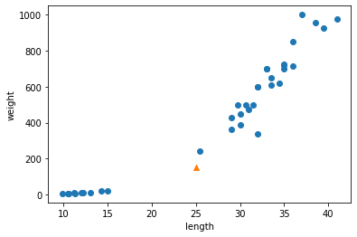
distances, indexes = kn.kneighbors([[25,150]]) # the nearest neighbors (default: 5)

# Scatter plot with 5 nearest neighbors
fig, ax = plt.subplots()
ax.scatter(train_input[:,0], train_input[:,1])
ax.scatter(25, 150, marker="^")
ax.scatter(train_input[indexes,0], train_input[indexes,1], marker='D') # rhombus marker
ax.set_xlabel('length')
ax.set_ylabel('weight')
plt.show()

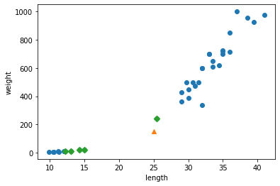
# Scatter plot on the same scale
fig, ax = plt.subplots()
ax.scatter(train_input[:,0], train_input[:,1])
ax.scatter(25, 150, marker="^")
ax.scatter(train_input[indexes,0], train_input[indexes,1], marker='D') # rhombus marker
ax.set_xlim((0,1000)) # change the x scale
ax.set_xlabel('length')
ax.set_ylabel('weight')
plt.show()

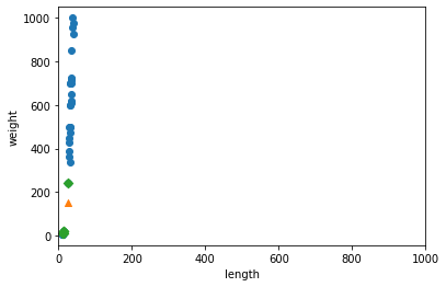
KNN 2

Data Preprocessing

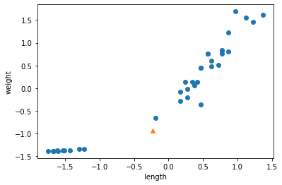
# standard score
mean = np.mean(train_input, axis=0) # axis=0 : for each feature
std = np.std(train_input, axis=0)
train_scaled = (train_input - mean) / std # broadcasting in numpy

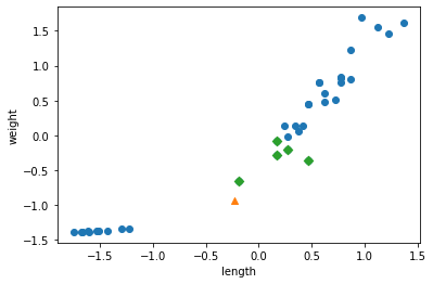
# Scatter plot with standard score
new = ([25, 150] - mean ) / std
fig, ax = plt.subplots()
ax.scatter(train_scaled[:,0], train_scaled[:,1])
ax.scatter(new[0], new[1], marker="^")
ax.set_xlabel('length')
ax.set_ylabel('weight')
plt.show()

KNN fitting

test_scaled = (test_input - mean) / std
kn.fit(train_scaled, train_target)
kn.score(test_scaled, test_target) # 

1.0

Predicting new data

print(kn.predict([new])) # the actual data is a bream, and predicted to be bream.

[1.]

distances, indexes = kn.kneighbors([new])

# Scatter plot with 5 nearest neighbors
fig, ax = plt.subplots()
ax.scatter(train_scaled[:,0], train_scaled[:,1])
ax.scatter(new[0], new[1], marker="^")
ax.scatter(train_scaled[indexes,0], train_scaled[indexes,1], marker='D') # rhombus marker
ax.set_xlabel('length')
ax.set_ylabel('weight')
plt.show()

Ref.) 혼자 공부하는 머신러닝+딥러닝 (박해선, 한빛미디어)